Activation Functions | ML Refresher

11.1 Why nonlinearity is needed

Without a nonlinearity, two layers collapse into one. For row vectors, $(\vx\mW_1+\vb_1)\mW_2+\vb_2 = \vx(\mW_1\mW_2)(\vb_1\mW_2\vb_2)$ . Depth would only refactor a matrix. A pointwise activation $a$ breaks that collapse: $\vh=a(\vx\mW_1+\vb_1)$ . Backprop needs its local slope, $\bar{\vz}=\bar{\vh}\odot a'(\vz)$ , so an activation is also a gate on the gradient.

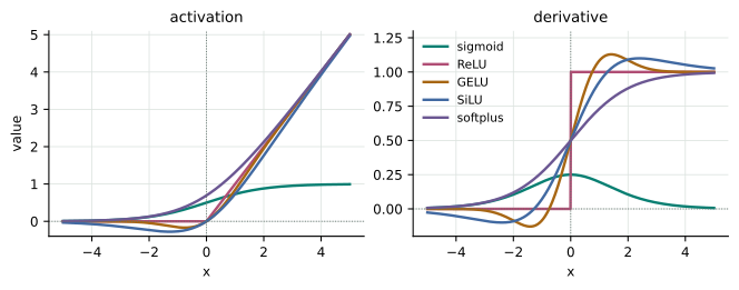
That gate is why activation choice shows up in training curves. If most local slopes are near zero, upstream layers learn slowly even when the loss is large. If the slopes are too large or too variable, gradients can grow as they pass through many layers. Useful activations therefore do two jobs at once: they let the network build nonlinear features, and they keep enough derivative mass near the values produced by normalized hidden states. The calculus chapter has an interactive lab for comparing these curves directly; see Chapter 3.

Activation functions and their derivatives

Figure 11.1 Common activation functions and their local slopes. Sigmoid saturates; ReLU is sparse; GELU and SiLU are smooth; softplus is a smooth ReLU.

11.2 Saturating and rectified activations

The logistic sigmoid and tanh are smooth squashing functions:

\sigma(x)=\frac{1}{1+e^{-x}}, \qquad \tanh x=2\sigma(2x)-1 .\tag{11.1}

Their derivatives follow by one line of algebra: $\frac{\mathrm{d}}{\mathrm{d}x}\frac{1}{1+e^{-x}} = \frac{e^{-x}}{(1+e^{-x})^2} = \sigma(x)(1-\sigma(x))$ , and $\tanh'(x)=1-\tanh^2(x)$ . Thus $0 \le \sigma'(x) \le 1/4$ and $0 \le \tanh'(x) \le 1$ . Far from zero both slopes approach 0, so early deep networks could lose gradients through saturated units [glorot2010].

Sigmoid is still the right shape when a value should behave like a probability or a soft gate. Tanh is centered at zero, which often makes it easier to optimize than sigmoid in hidden states, but it saturates just as surely. The derivative bounds are useful sanity checks in backprop: a chain of many saturated sigmoids multiplies many numbers smaller than $1/4$ . That is not a subtle numerical problem; it is a direct consequence of the derivative.

ReLU replaces saturation on the positive side with a kink:

\operatorname{ReLU}(x)=\max(x,0), \qquad \operatorname{ReLU}'(x)=\mathbf{1}\{x>0\} .\tag{11.2}

It is cheap and sparse [nair2010], but a unit whose pre-activation stays negative has zero output and zero gradient: a dead unit. Leaky ReLU changes the left slope to a small $\alpha$ , $a(x)=\max(x,\alpha x)$ , so negative inputs still receive gradient $\alpha$ . At $x=0$ these rectifiers are not differentiable; implementations choose a subgradient, and our tests avoid the kink for finite differences.

The subgradient choice at one point almost never matters for random continuous inputs. The zero half-line matters much more. ReLU’s exact zeros make activations sparse and cheap to reason about, but they also mean a bad bias or a large update can put a unit on the wrong side of the kink for every example. Leaky ReLU trades away exact sparsity for a small escape route.

Listing 11.1 Elementwise activations and derivatives

def sigmoid(x):
    x = np.asarray(x)
    positive = x >= 0
    z = np.exp(-np.abs(x))
    return np.where(positive, 1 / (1 + z), z / (1 + z))


def sigmoid_grad(x):
    y = sigmoid(x)
    return y * (1 - y)


def tanh_grad(x):
    y = np.tanh(x)
    return 1 - y * y


def relu(x):
    return np.maximum(x, 0)


def relu_grad(x):
    return (np.asarray(x) > 0).astype(float)


def leaky_relu(x, negative_slope=0.01):
    return np.where(np.asarray(x) >= 0, x, negative_slope * np.asarray(x))


def leaky_relu_grad(x, negative_slope=0.01):
    return np.where(np.asarray(x) >= 0, 1.0, negative_slope)

11.3 Smooth activations

GELU gates an input by the probability that a standard normal variable is below it [hendrycks2016gaussian]:

\operatorname{GELU}(x)=x\Phi(x), \qquad \operatorname{GELU}'(x)=\Phi(x)+x\phi(x) .\tag{11.3}

The derivative is the product rule; $\Phi'(x)=\phi(x)$ . Many implementations use the tanh approximation $0.5x(1+\tanh(\sqrt{2/\pi}(x+0.044715x^3)))$ . On a 200,001-point grid over $[-8,8]$ , the chapter test measures a maximum absolute error of $4.7324\times10^{-4}$ .

The intuition is a soft version of dropout by value: strongly positive inputs pass almost unchanged, strongly negative inputs are almost removed, and values near zero pass partly. GELU is smooth at zero, unlike ReLU, so its derivative changes continuously. The tanh approximation exists because $\Phi$ involves the error function; the approximation keeps the shape while using only elementary operations common in accelerator kernels.

Listing 11.2 GELU exactly and with the tanh approximation

def normal_pdf(x):
    return _INV_SQRT_2PI * np.exp(-0.5 * np.asarray(x) ** 2)


def normal_cdf(x):
    return 0.5 * (1 + _erf(np.asarray(x) / _SQRT_2))


def gelu_exact(x):
    x = np.asarray(x)
    return x * normal_cdf(x)


def gelu_exact_grad(x):
    x = np.asarray(x)
    return normal_cdf(x) + x * normal_pdf(x)


def gelu_tanh(x):
    x = np.asarray(x)
    u = _SQRT_2_OVER_PI * (x + _GELU_COEFF * x ** 3)
    return 0.5 * x * (1 + np.tanh(u))


def gelu_tanh_grad(x):
    x = np.asarray(x)
    u = _SQRT_2_OVER_PI * (x + _GELU_COEFF * x ** 3)
    du = _SQRT_2_OVER_PI * (1 + 3 * _GELU_COEFF * x ** 2)
    sech2 = 1 - np.tanh(u) ** 2
    return 0.5 * (1 + np.tanh(u)) + 0.5 * x * sech2 * du

SiLU, also called Swish, is $x\sigma(x)$ [ramachandran2017searching]. Its derivative is $\sigma(x)x\sigma(x)(1-\sigma(x))]. Softplus is the smooth ReLU, stem:[\log(1+e^x)], and its derivative is exactly stem:[\sigma(x)]. The stable implementation uses stem:[\max(x,0)\log(1+e^{-|x|})$ so large positive inputs do not overflow.

SiLU is slightly nonmonotone on the negative side, which lets small negative evidence survive instead of being clipped exactly to zero. Softplus is most useful when a model must produce a positive number, such as a scale parameter, while still remaining differentiable everywhere. For large positive $x$ , softplus is almost $x$ ; for large negative $x$ , it is almost $0$ . Its derivative being sigmoid makes that transition explicit.

Listing 11.3 SiLU and softplus

def silu(x):
    x = np.asarray(x)
    return x * sigmoid(x)


def silu_grad(x):
    x = np.asarray(x)
    s = sigmoid(x)
    return s + x * s * (1 - s)


def softplus(x):
    x = np.asarray(x)
    return np.maximum(x, 0) + np.log1p(np.exp(-np.abs(x)))


def softplus_grad(x):
    return sigmoid(x)

11.4 Gated feed-forward blocks

A Transformer feed-forward block applies an activation between two linear maps. A width $4d$ MLP has about $d(4d)+(4d)d=8d^2$ weights. A gated block uses two input projections and one output projection,

\operatorname{FFN}(\vx) = \big(a(\vx\mW) \odot \vx\mV\big)\mW_2 .\tag{11.4}

Its count is $d h+d h+h d=3d h$ . Matching the $4d$ MLP therefore sets $3dh=8d^2$ , or $h=8d/3$ . In practice that width is rounded to a hardware-friendly multiple. GLU, ReGLU, GeGLU, and SwiGLU use $a=\sigma$ , ReLU, GELU, and SiLU respectively; the elementwise product lets one projection gate the other [shazeer2020glu].

The formula uses the prompt’s convention: the activated projection is the gate and the second projection carries the values. Some libraries swap the two names, but multiplication is commutative, so the block is the same after renaming $\mW$ and $\mV$ . Biases and rounding change the exact count by lower-order terms; the $8d/3$ rule is the leading comparison that keeps a gated block near the budget of the familiar $4d$ MLP.

The backward pass is just the product rule. If $\vg=\bar{\vy}\mW_2^\T$ , then $\bar{\vu}=\vg\odot a(\vz)$ and $\bar{\vz}=\vg\odot\vu\odot a'(\vz)$ , where $\vz=\vx\mW$ and $\vu=\vx\mV$ . The test suite checks the resulting parameter gradients by finite differences.

This is the only extra backprop idea in the GLU family. The output projection backpropagates into the product; the product sends one factor’s gradient through the other factor; and the activation derivative is applied only on the gated branch. Once that is in place, GLU, ReGLU, GeGLU, and SwiGLU differ only by the choice of $a$ and $a'$ .

Listing 11.4 Gated GLU-family feed-forward block

def gated_ffn(x, W, V, W2, kind="swiglu"):
    """(act(x @ W) * (x @ V)) @ W2, with rows as examples."""
    act, _ = _ACTIVATIONS[kind]
    return (act(x @ W) * (x @ V)) @ W2


def gated_ffn_backward(x, W, V, W2, grad_y, kind="swiglu"):
    act, act_grad = _ACTIVATIONS[kind]
    z, u = x @ W, x @ V
    a, h = act(z), act(z) * u
    grad_W2 = h.T @ grad_y
    grad_h = grad_y @ W2.T
    grad_z = grad_h * u * act_grad(z)
    grad_u = grad_h * a
    grad_W = x.T @ grad_z
    grad_V = x.T @ grad_u
    grad_x = grad_z @ W.T + grad_u @ V.T
    return grad_x, grad_W, grad_V, grad_W2

In practice

Sigmoid and tanh are still useful as gates and output squashes, but hidden layers in LLMs use rectified or smooth activations. GELU became common in Transformer encoders, while PaLM used SwiGLU in its feed-forward blocks [chowdhery2022palm]. Shazeer reports that GLU variants, especially GeGLU and SwiGLU, improve Transformer quality at comparable parameter counts [shazeer2020glu]. The important engineering point is not the exact curve; it is keeping activation scales and derivative scales friendly to deep backpropagation.

Key equations

\sigma'(x)=\sigma(x)(1-\sigma(x)), \qquad \tanh'(x)=1-\tanh^2(x)

\operatorname{ReLU}'(x)=\mathbf{1}\{x>0\}, \qquad \operatorname{softplus}'(x)=\sigma(x)

\operatorname{GELU}(x)=x\Phi(x), \qquad \operatorname{GELU}'(x)=\Phi(x)+x\phi(x)

\operatorname{SiLU}(x)=x\sigma(x), \qquad \operatorname{SiLU}'(x)=\sigma(x)+x\sigma(x)(1-\sigma(x))

\operatorname{FFN}(\vx)=(a(\vx\mW)\odot\vx\mV)\mW_2, \qquad h=8d/3

11.5 Teach it

The one-sentence version. An activation is a pointwise bend in the network; its value gates features forward and its derivative gates gradients backward.

An analogy. Linear layers are like transparent sheets with grids printed on them. Stacking sheets only makes another grid. An activation bends the sheet, so the next grid sees a new shape.

At the board.

Multiply two affine maps and show they collapse into one.
Draw sigmoid and ReLU slopes: sigmoid saturates; ReLU can die on the left.
Derive GELU’s derivative with the product rule, $(x\Phi(x))'=\Phi(x)+x\phi(x)$ .
Count gated FFN parameters: two $d\times h$ projections plus one $h\times d$ .

Misconceptions to address.

"More nonlinear is always better." Too much saturation kills gradients.
"ReLU has no derivative." It has one away from zero; the kink uses a chosen subgradient.
"SwiGLU is a new matrix shape." It is an activation choice inside a gated FFN.

Check for understanding. Why does a gated FFN with $h=4d$ have more parameters than a plain $4d$ MLP?

11.6 Exercises

Exercise 11.1 ★ Saturation and dead units

Explain why the derivatives of sigmoid and tanh vanish for large $|x|$ . Then explain why ReLU can create dead units and how leaky ReLU changes the gradient.

Solution in Appendix D

Exercise 11.2 ★★ Derivatives by hand

Derive $\sigma'(x)$ , $\tanh'(x)$ , $\operatorname{SiLU}'(x)$ , and $\operatorname{softplus}'(x)$ . State the maximum derivative of sigmoid and tanh.

Solution in Appendix D

Exercise 11.3 ★★ GELU exact versus approximate

Derive $(x\Phi(x))'$ . Then measure the maximum absolute error of the tanh approximation on $[-8,8]$ using gelu_tanh_max_error.

Solution in Appendix D

Exercise 11.4 ★★★ Matching gated-FFN parameters

A plain Transformer MLP maps $d \to 4d \to d$ . A gated GLU-family block maps $d \to h$ twice, multiplies the two hidden vectors elementwise, and maps $h \to d$ . Derive $h=8d/3$ , and gradient-check the gated block’s backward pass for a tiny matrix.

Solution in Appendix D

References

[glorot2010] X. Glorot and Y. Bengio. Understanding the difficulty of training deep feedforward neural networks. AISTATS 2010.
[nair2010] V. Nair and G. E. Hinton. Rectified linear units improve restricted Boltzmann machines. ICML 2010.
[chowdhery2022palm] A. Chowdhery et al. PaLM: Scaling Language Modeling with Pathways. 2022. arXiv:2204.02311
[hendrycks2016gaussian] D. Hendrycks and K. Gimpel. Gaussian Error Linear Units (GELUs). 2016. arXiv:1606.08415
[ramachandran2017searching] P. Ramachandran, B. Zoph, and Q. V. Le. Searching for Activation Functions. 2017. arXiv:1710.05941
[shazeer2020glu] N. Shazeer. GLU Variants Improve Transformer. 2020. arXiv:2002.05202