Information Theory | ML Refresher

7.1 Surprisal

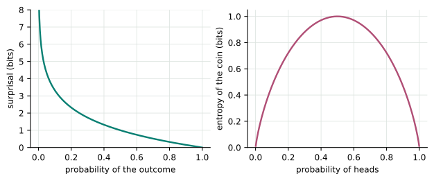
An outcome with probability $p$ carries some amount of information, or surprisal $I(p)$ . Three requirements pin down what $I$ must be. A certain event carries no information, $I(1) = 0$ . Rarer events are more surprising, so $I$ decreases as $p$ grows. Most importantly, the information of two independent outcomes should add: $I(pq) = I(p) + I(q)$ . The only continuous functions that turn products into sums are logarithms, so

I(x) = -\log p(x) .\tag{7.1}

The base of the logarithm sets the unit. Base 2 measures bits, and the natural logarithm measures nats: one nat is $1 / \ln 2 \approx 1.44$ bits. A fair coin flip carries 1 bit. A fair die roll carries $\log_2 6 \approx 2.58$ bits. One specific token drawn uniformly from a 128,000-token vocabulary carries about 17 bits. The whole book uses nats unless it says otherwise, because that is what np.log computes.

7.2 Entropy

Entropy is the expected surprisal of a random variable, its average information per outcome:

H(p) = \E_{x \sim p}[-\log p(x)] = -\sum_x p(x) \log p(x) ,\tag{7.2}

with the convention $0 \log 0 = 0$ , the limit of $t \log t$ as $t \to 0$ . Entropy measures uncertainty. It is 0 for a certain outcome and largest for the uniform distribution over $K$ values, where it equals $\log K$ (Exercise 7.2). A coin with heads probability $p$ has entropy $-p \log p - (1-p)\log(1-p)$ , which peaks at one bit for a fair coin.

Figure 7.1 Left: the surprisal of one outcome grows without bound as its probability falls. Right: a coin’s entropy, the average surprisal of a flip, peaks at one bit when heads and tails are equally likely.

Entropy also has a concrete meaning, from Shannon’s source coding theorem [shannon1948]. To transmit outcomes drawn from $p$ in binary, no lossless code can use fewer than $H(p)$ bits per outcome on average. Codes that give outcome $x$ about $-\log_2 p(x)$ bits come close. Take four symbols with probabilities $\tfrac12, \tfrac14, \tfrac18, \tfrac18$ and the prefix code 0, 10, 110, 111. Each codeword is exactly $-\log_2 p$ bits long, and the average is $\tfrac12 \cdot 1 + \tfrac14 \cdot 2 + \tfrac18 \cdot 3 + \tfrac18 \cdot 3 = 1.75$ bits: precisely the entropy.

The shared scratch package computes entropy with the $0 \log 0$ convention built in, alongside the next two quantities of this chapter:

Listing 7.1 Entropy, cross-entropy, and KL divergence

def entropy(p, axis=-1):
    """H(p) = -sum p log p, in nats, with the convention 0 log 0 = 0."""
    p = np.asarray(p, dtype=np.float64)
    safe = np.where(p > 0, p, 1.0)                  # log(1) = 0 where p = 0
    return -np.sum(p * np.log(safe), axis=axis)


def cross_entropy(p, q, axis=-1):
    """H(p, q) = -sum p log q: infinite when q = 0 somewhere that p > 0."""
    p, q = np.asarray(p, dtype=np.float64), np.asarray(q, dtype=np.float64)
    with np.errstate(divide="ignore"):
        log_q = np.where(p > 0, np.log(q), 0.0)
    return -np.sum(p * log_q, axis=axis)


def kl_divergence(p, q, axis=-1):
    """KL(p || q) = sum p log(p / q), computed directly, not as H(p, q) - H(p)."""
    p, q = np.asarray(p, dtype=np.float64), np.asarray(q, dtype=np.float64)
    with np.errstate(divide="ignore"):
        log_ratio = np.where(p > 0, np.log(np.where(p > 0, p, 1.0)) - np.log(q), 0.0)
    return np.sum(p * log_ratio, axis=axis)

7.3 Cross-entropy

Suppose the data come from $p$ , but we encode them with a code designed for a different distribution $q$ . Each outcome then costs $-\log q(x)$ , and the average cost is the cross-entropy:

H(p, q) = \E_{x \sim p}[-\log q(x)] = -\sum_x p(x) \log q(x) .\tag{7.3}

Encoding the four symbols above with a uniform code, two bits each, costs $H(p, q) = 2$ bits per symbol instead of 1.75. The extra 0.25 bits are the price of using the wrong distribution. In machine learning, $p$ is the data and $q$ is the model, and the cross-entropy measures how many nats per outcome the model needs to describe the data.

Cross-entropy is not symmetric, and it is infinite if $q(x) = 0$ for any $x$ that $p$ can produce. A model that assigns zero probability to something that happens pays an unbounded price. That is one reason models output probabilities through a softmax, which is never exactly zero.

7.4 KL divergence

The Kullback–Leibler divergence is the extra cost itself [kullback1951]:

\KL(p \,\Vert\, q) = \sum_x p(x) \log \frac{p(x)}{q(x)} = H(p, q) - H(p) .\tag{7.4}

In the coding example it is exactly 0.25 bits. Its central property, Gibbs' inequality, is that it is never negative, and it is zero only when $q = p$ :

\KL(p \,\Vert\, q) \ge 0, \quad\text{with equality if and only if } p = q .\tag{7.5}

The proof is one application of Jensen’s inequality to the concave logarithm (Exercise 7.3). It follows that $H(p, q) \ge H(p)$ : no model describes data more cheaply than the true distribution.

KL divergence is often called a distance, but it is not one. It is not symmetric, and it does not satisfy the triangle inequality. The asymmetry is the point. $\KL(p \Vert q)$ averages over $p$ , so it punishes $q$ heavily wherever $p$ has mass that $q$ lacks. $\KL(q \Vert p)$ averages over $q$ , so it punishes $q$ wherever it puts mass that $p$ lacks.

For two univariate Gaussians the divergence has a closed form, which reappears in variational autoencoders and in KL penalties on Gaussian policies:

\KL\big(\mathcal{N}(\mu_1, \sigma_1^2) \,\Vert\, \mathcal{N}(\mu_2, \sigma_2^2)\big) = \log \frac{\sigma_2}{\sigma_1} + \frac{\sigma_1^2 + (\mu_1 - \mu_2)^2}{2\sigma_2^2} - \frac12 .\tag{7.6}

Listing 7.2 The Gaussian KL divergence in closed form

def gaussian_kl(mean_p, std_p, mean_q, std_q):
    """KL(N(mean_p, std_p^2) || N(mean_q, std_q^2)) in closed form."""
    return (np.log(std_q / std_p)
            + (std_p ** 2 + (mean_p - mean_q) ** 2) / (2 * std_q ** 2) - 0.5)

7.4.1 Forward and reverse KL

The asymmetry becomes vivid when we approximate a complicated distribution $p$ with a simple family. Take a target with two separated modes, and fit a single Gaussian $q$ by searching over its mean and standard deviation:

Listing 7.3 Fitting a Gaussian by minimizing either direction of KL

def kl_on_grid(p, q):
    """KL(p || q) for densities sampled on GRID: a Riemann sum of p log(p / q)."""
    inside = p > 1e-300
    with np.errstate(divide="ignore"):              # q = 0 where p > 0: KL is infinite
        log_ratio = np.log(p[inside]) - np.log(q[inside])
    return np.sum(p[inside] * log_ratio) * STEP


def fit_gaussian(target, direction, means, stds):
    """Find the Gaussian q minimizing KL(p||q) or KL(q||p)."""
    p = target(GRID)
    best = (np.inf, None, None)
    for mean in means:
        for std in stds:
            q = gaussian_density(GRID, mean, std)
            forward = direction == "forward"
            divergence = kl_on_grid(p, q) if forward else kl_on_grid(q, p)
            best = min(best, (divergence, mean, std), key=lambda item: item[0])
    return best[1], best[2]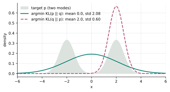

A two-mode target with a broad forward-KL fit and a narrow reverse-KL fit

Figure 7.2 Minimizing the forward KL

\KL(p \Vert q)

spreads

q

over both modes. Minimizing the reverse KL

\KL(q \Vert p)

makes

q

commit to a single mode.

Forward KL is mass-covering: any region where $p > 0$ and $q \approx 0$ costs a fortune, so $q$ stretches over both modes, even though that puts most of its own mass in the empty valley between them. For Gaussian $q$ , the optimum matches the mean and variance of $p$ . Here that means mean 0 and standard deviation $\sqrt{0.6^2 + 2^2} \approx 2.09$ (Exercise 7.7). Reverse KL is mode-seeking: $q$ is only penalized where it puts mass, so it settles on one mode, mean $\pm 2$ and standard deviation 0.6, and ignores the other entirely.

Both directions appear in practice [bishop2006]. Maximum-likelihood training, supervised fine-tuning, and classical distillation minimize the forward KL from the data or teacher to the model, so the model tries to cover everything the data does. Variational inference, the KL penalty in RLHF, and on-policy distillation use the reverse direction, measured on samples from the model itself.

7.5 Cross-entropy is maximum likelihood

Given training samples $x_1, \dots, x_N$ , let $\hat{p}$ be their empirical distribution, the fraction of samples equal to each value. The average negative log-likelihood of a model $q_\vtheta$ (Section 6.5) rewrites exactly as a cross-entropy:

-\frac{1}{N}\sum_{i=1}^{N} \log q_\vtheta(x_i) = -\sum_x \hat{p}(x) \log q_\vtheta(x) = H(\hat{p}, q_\vtheta) = H(\hat{p}) + \KL(\hat{p} \,\Vert\, q_\vtheta) .\tag{7.7}

$H(\hat{p})$ does not depend on the model. Maximizing likelihood, minimizing cross-entropy, and minimizing the forward KL from the data to the model are therefore three names for one optimization. This is why a classifier’s loss is called "cross-entropy" and a language model’s pretraining loss is reported in nats or bits per token.

Listing 7.4 The maximum-likelihood objective is a cross-entropy

def empirical_distribution(samples, categories):
    """The fraction of samples equal to each category: p_hat."""
    return np.bincount(samples, minlength=categories) / len(samples)


def average_nll(samples, q):
    """The maximum-likelihood objective: -(1/N) sum_i log q(x_i)."""
    return float(-np.mean(np.log(q[samples])))


def cross_entropy_of_empirical(samples, q):
    """The same number, as the cross-entropy H(p_hat, q)."""
    return float(cross_entropy(empirical_distribution(samples, len(q)), q))

7.6 Perplexity

A language model assigns each token of a held-out text a log-probability. Their negative average is the cross-entropy per token. Perplexity is its exponential:

\operatorname{PPL} = \exp\Big(-\frac{1}{T} \sum_{t=1}^{T} \log q_\vtheta(x_t \mid x_{<t})\Big) .\tag{7.8}

Perplexity is the size of a uniform distribution with the same cross-entropy: the model is as uncertain as if it were choosing uniformly among PPL tokens at every step. A model that guesses uniformly over a 50,000-token vocabulary has perplexity 50,000, and a model that is always certain and always right has perplexity 1. Dividing the cross-entropy by $\ln 2$ gives bits per token. Neither number can be compared across tokenizers without care: a tokenizer with longer tokens has fewer, harder predictions.

Listing 7.5 Perplexity and bits per token from token log-probabilities

def perplexity(token_log_probs):
    """exp of the average negative log-likelihood per token (natural logs)."""
    return float(np.exp(-np.mean(token_log_probs)))


def bits_per_token(token_log_probs):
    """The same average, measured in bits."""
    return float(-np.mean(token_log_probs) / np.log(2))

7.7 Mutual information

How much does knowing $Y$ tell us about $X$ ? The mutual information compares the joint distribution with the product of the marginals, the distribution the pair would have if the variables were independent:

\begin{aligned} I(X; Y) &= \KL\big(p(x, y) \,\Vert\, p(x)\,p(y)\big) \\ &= H(X) + H(Y) - H(X, Y) = H(X) - H(X \mid Y) . \end{aligned}\tag{7.9}

It is zero exactly when $X$ and $Y$ are independent, and it equals $H(X)$ when $Y$ determines $X$ . For the joint table used in the tests, $\left(\begin{smallmatrix} 0.30 & 0.10 \\ 0.15 & 0.45 \end{smallmatrix}\right)$ , the mutual information is 0.126 nats (0.18 bits). Knowing $X$ removes about 18% of the uncertainty in $Y$ :

Listing 7.6 Mutual information, two ways

def mutual_information(joint):
    """I(X; Y) = KL(p(x, y) || p(x) p(y)) for a joint probability table."""
    px, py = joint.sum(axis=1), joint.sum(axis=0)
    return float(kl_divergence(joint.ravel(), np.outer(px, py).ravel()))


def mutual_information_from_entropies(joint):
    """The same quantity as H(X) + H(Y) - H(X, Y)."""
    marginal_x, marginal_y = joint.sum(axis=1), joint.sum(axis=0)
    return float(entropy(marginal_x) + entropy(marginal_y) - entropy(joint.ravel()))

Contrastive learning, including CLIP, maximizes a lower bound on the mutual information between two views of the same data [oord2018]. Its loss, InfoNCE, is a cross-entropy in disguise.

7.8 Estimating KL from samples

In reinforcement learning from human feedback, the policy $q$ being trained is kept close to a reference model $p$ by penalizing $\KL(q \Vert p)$ . Summing over every possible response is impossible, but we can sample responses from $q$ and evaluate both models' log-probabilities on them. With $r = p(x) / q(x)$ and $x \sim q$ , three per-sample estimators are common [schulman2020]:

k_1 = -\log r, \qquad k_2 = \tfrac12 (\log r)^2, \qquad k_3 = (r - 1) - \log r .\tag{7.10}

$k_1$ is unbiased, because $\E_q[-\log r] = \KL(q \Vert p)$ . However, it is negative for many samples, and its variance is large. $k_2$ is always nonnegative but biased. $k_3$ adds $r - 1$ , which has expectation zero under $q$ , so it is still unbiased. It is also never negative (Exercise 7.6). GRPO uses $k_3$ as its KL penalty [shao2024].

Listing 7.7 Three estimators of KL divergence from samples

def kl_estimators(log_p, log_q):
    """Per-sample estimates of KL(q || p) from draws x ~ q.

    Each argument holds log p(x) or log q(x) at the same draws. With r = p(x) / q(x):
    k1 = -log r, k2 = (log r)^2 / 2, and k3 = (r - 1) - log r.
    """
    log_r = log_p - log_q
    k1 = -log_r
    k2 = 0.5 * log_r ** 2
    k3 = np.expm1(log_r) - log_r
    return k1, k2, k3

Take $q = \mathcal{N}(0, 1)$ and $p = \mathcal{N}(0.1, 1)$ , so $\KL(q \Vert p) = 0.005$ . Over a million samples, the standard deviation of $k_1$ is 20 times the divergence itself, while that of $k_3$ is 1.42 times. When $p = \mathcal{N}(1, 1)$ and the divergence is 0.5, $k_2$ overestimates it by 25%, while $k_3$ remains unbiased.

In practice

Every quantity in this chapter is computed daily in training. Pretraining minimizes cross-entropy and reports perplexity. Label smoothing mixes the one-hot target with a uniform distribution before the cross-entropy. Distillation minimizes a KL divergence between teacher and student distributions. RLHF and GRPO add a per-token KL penalty toward a reference model, estimated from the policy’s own samples. The entropy of the policy’s next-token distribution is monitored during reinforcement learning because a sudden collapse toward zero signals lost exploration. Treat the direction of every KL you meet as a design decision.

Key equations

I(x) = -\log p(x), \qquad H(p) = -\sum_x p(x)\log p(x) \le \log K

H(p, q) = -\sum_x p(x) \log q(x) = H(p) + \KL(p \Vert q), \qquad \KL(p \Vert q) = \sum_x p(x)\log\frac{p(x)}{q(x)} \ge 0

-\frac1N\sum_i \log q_\vtheta(x_i) = H(\hat{p}, q_\vtheta), \qquad \operatorname{PPL} = \exp(\text{cross-entropy per token})

I(X; Y) = \KL(p(x, y) \Vert p(x)p(y)) = H(X) - H(X \mid Y)

\KL(q \Vert p) = \E_{x \sim q}\big[(r - 1) - \log r\big], \quad r = p(x)/q(x)

7.9 Teach it

The one-sentence version. Surprise is minus the log-probability. Entropy is average surprise. Cross-entropy is average surprise when you believe the wrong distribution. KL divergence is the difference: the price of believing wrongly.

An analogy. Twenty questions. With a good strategy, the number of yes-or-no questions you need to identify an outcome is its surprisal in bits, and the average number is the entropy. If you plan your questions around the wrong beliefs, you need more questions on average. The extra questions are the KL divergence.

At the board.

Write the four-symbol code 0, 10, 110, 111 beside the probabilities $\tfrac12, \tfrac14, \tfrac18, \tfrac18$ . Compute the average length, 1.75 bits, and then the entropy.
Now use a two-bit code for every symbol. The average becomes 2 bits, the cross-entropy, and the 0.25-bit gap is the KL divergence.
Write the average negative log-likelihood of a dataset and rewrite it as a sum over values weighted by their frequencies. It becomes a cross-entropy with the empirical distribution.
Sketch two humps and ask the room to fit one Gaussian. Forward KL spans both humps; reverse KL hugs one.

Misconceptions to address.

"KL divergence is a distance." It is not symmetric, and the direction matters.
"Lower perplexity always means a better model." Only for the same tokenizer and test data.
"Cross-entropy and log-loss are different losses." They are the same quantity.
"Entropy is a property of a single outcome." It is a property of a distribution; surprisal belongs to an outcome.

Check for understanding. A model assigns probability 0 to a token that appears in the test set. What is its perplexity, and what does that say about using a softmax output?

7.10 Exercises

Exercise 7.1 ★ Counting bits

Compute the surprisal, in bits and in nats, of a fair coin landing heads, a fair die showing six, and one specific token drawn uniformly from a 128,000-token vocabulary.

Solution in Appendix D

Exercise 7.2 ★ The most uncertain distribution

Show that $\log K - H(p) = \KL(p \Vert u)$ , where $u$ is the uniform distribution on $K$ values. Conclude that $H(p) \le \log K$ , with equality only for the uniform distribution.

Solution in Appendix D

Exercise 7.3 ★★ Gibbs' inequality

Prove (7.5) using Jensen’s inequality, $\E[\log Z] \le \log \E[Z]$ for a positive random variable $Z$ , with equality only when $Z$ is constant.

Solution in Appendix D

Exercise 7.4 ★★ Likelihood as cross-entropy

Derive (7.7). Then explain why a model trained by maximum likelihood on a finite dataset is pushed toward the empirical distribution, and what could stop it from reaching it.

Solution in Appendix D

Exercise 7.5 ★★ KL between Gaussians

Derive (7.6) by writing the log-ratio of the two densities and taking its expectation under the first. Check that the result is zero when the Gaussians are equal, and that it grows quadratically in the distance between the means.

Solution in Appendix D

Exercise 7.6 ★★ An unbiased, nonnegative estimator

With $r = p(x)/q(x)$ and $x \sim q$ , show that $\E_q[r] = 1$ , so that $\E_q[k_3] = \KL(q \Vert p)$ . Then show that $k_3 \ge 0$ for every $r > 0$ .

Solution in Appendix D

Exercise 7.7 ★★★ Forward KL matches moments

Show that among all Gaussians $q$ , the minimizer of $\KL(p \Vert q)$ has the same mean and variance as $p$ . Hint: only $-\E_p[\log q]$ depends on $q$ . Verify this numerically with fit_gaussian, and explain why the reverse direction has no such simple answer.

Solution in Appendix D

Exercise 7.8 ★★★ Mutual information three ways

For the joint table $\left(\begin{smallmatrix} 0.30 & 0.10 \\ 0.15 & 0.45 \end{smallmatrix}\right)$ , compute $I(X; Y)$ as a KL divergence, from entropies, and as $H(Y) - H(Y \mid X)$ . Then compute it for a table in which $Y = X$ always, and for the product of the marginals.

Solution in Appendix D

References

[bishop2006] C. M. Bishop. Pattern Recognition and Machine Learning. Springer, 2006.
[cover2006] T. M. Cover and J. A. Thomas. Elements of Information Theory, 2nd edition. Wiley, 2006.
[kullback1951] S. Kullback and R. A. Leibler. On information and sufficiency. Annals of Mathematical Statistics 22(1), 79–86, 1951.
[mackay2003] D. J. C. MacKay. Information Theory, Inference, and Learning Algorithms. Cambridge University Press, 2003. https://www.inference.org.uk/mackay/itila/
[oord2018] A. van den Oord, Y. Li, and O. Vinyals. Representation learning with contrastive predictive coding. 2018. arXiv:1807.03748
[schulman2020] J. Schulman. Approximating KL divergence. Blog post, 2020. http://joschu.net/blog/kl-approx.html
[shannon1948] C. E. Shannon. A mathematical theory of communication. Bell System Technical Journal 27, 379–423 and 623–656, 1948.
[shao2024] Z. Shao et al. DeepSeekMath: Pushing the limits of mathematical reasoning in open language models. 2024. arXiv:2402.03300