Chapter 44

Capstone: An LLM End to End

Tokenizer, pretraining, fine-tuning, preference training, decoding, and a tool-using agent.

Each chapter built one part of a language model. This one puts them in order. It also sizes a real model with the book’s rules of thumb, and gives a test for each stage you build. Use it as a map when building, and as a syllabus when teaching.

44.1 The pipeline

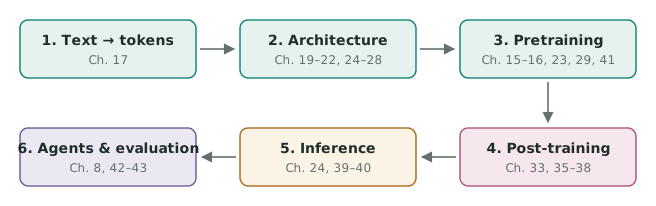
Figure 44.1 Six stages turn text into a working assistant. Each box lists the chapters that build it.

Text to tokens. Clean, deduplicated text is split into bytes and merged into subword tokens by byte-level BPE (Chapter 17).
Architecture. Token embeddings pass through $L$ pre-norm blocks. Each block applies causal multi-head attention with RoPE, then a SwiGLU feed-forward layer, each with RMSNorm and a residual connection. A tied output head and a softmax follow (Chapter 19, Chapter 20, Chapter 21, Chapter 22). Grouped-query or latent attention shrinks the KV cache, and mixture-of-experts layers add parameters without adding per-token compute (Chapter 24, Chapter 25, Chapter 27).
Pretraining. Minimize next-token cross-entropy (Chapter 18) with AdamW or Muon and a warmup-then-decay schedule (Chapter 15). Use bf16 arithmetic (Chapter 16), at a compute-optimal size (Chapter 29), sharded across devices (Chapter 41). Chapter 23 does all of it at toy scale.
Post-training. First, supervised fine-tuning on conversations, with the loss masked to the assistant’s tokens (Chapter 33). Then preferences, through a reward model with PPO or directly with DPO (Chapter 35, Chapter 36). Then reinforcement learning from verifiable rewards with GRPO (Chapter 37). Finally, distillation into smaller models (Chapter 38).
Inference. Prefill the prompt, then decode token by token from a KV cache, sampling with a temperature and truncation (Chapter 39). Quantize the weights and batch requests continuously (Chapter 40).
Agents and evaluation. Call tools in a loop, retrieve context, and measure everything with confidence intervals rather than single numbers (Chapter 42, Chapter 43, Chapter 8).

44.2 Sizing a model

Five formulas from earlier chapters size a model before any code runs. A pre-norm block with $H$ query heads, $H_\text{kv}$ key-value heads of width $d_h = d/H$ , and a SwiGLU feed-forward of width $8d/3$ has

N \approx L\big(2d^2 + 2 d H_\text{kv} d_h + 8d^2\big) + V d\tag{44.1}

parameters with a tied embedding of vocabulary $V$ . Training on $D$ tokens costs $C \approx 6ND$ FLOPs. The Chinchilla rule of thumb sets $D \approx 20N$ [hoffmann2022training]. Mixed-precision Adam holds about 16 bytes per parameter, and the KV cache of one sequence of $T$ tokens holds $2 L H_\text{kv} d_h T$ values:

\begin{aligned} C &\approx 6ND, \qquad D \approx 20N, \qquad M_\text{train} \approx 16N \text{ bytes} \\ M_\text{KV} &= 2\, L\, H_\text{kv}\, d_h\, T \cdot \text{bytes per value} \end{aligned}\tag{44.2}

Listing 44.1 The budget formulas

def transformer_parameters(layers, width, heads, kv_heads, vocabulary, tied=True):
    """Weights of a pre-norm decoder stack; norms and biases are ignored."""
    head_width = width // heads
    attention = 2 * width * width + 2 * width * kv_heads * head_width  # Q, O; K, V
    feed_forward = 8 * width * width            # a 4d MLP, or SwiGLU at width 8d/3
    embeddings = vocabulary * width * (1 if tied else 2)
    return layers * (attention + feed_forward) + embeddings


def training_flops(parameters, tokens):
    return 6 * parameters * tokens              # 2ND forward + 4ND backward


def compute_optimal_tokens(parameters, tokens_per_parameter=20):
    return tokens_per_parameter * parameters    # the Chinchilla rule of thumb


def training_memory_bytes(parameters):
    # bf16 weights and gradients (2 + 2), fp32 master copy (4), two Adam moments (4 + 4)
    return 16 * parameters


def kv_cache_bytes(layers, kv_heads, head_width, tokens, bytes_per_value=2):
    return 2 * layers * kv_heads * head_width * tokens * bytes_per_value

Take $L = 16$ , $d = 2048$ , 16 query heads, 4 key-value heads, and a 32,768-token vocabulary. The model has 771.8 million parameters. Compute-optimal training wants 15.4 billion tokens, or $7.15 \times 10^{19}$ FLOPs: 2.07 days at a sustained 400 TFLOP/s. Weights, gradients, and optimizer state need 12.3 GB before activations. A 4,096-token sequence needs a 128 MiB KV cache in bf16, a quarter of the 512 MiB that full multi-head attention would need.

Listing 44.2 Sizing the example model

def size_example(sustained_flops=400e12, context=4096):
    """Size the example model and its training run."""
    n = transformer_parameters(**EXAMPLE)
    d = compute_optimal_tokens(n)
    head_width = EXAMPLE["width"] // EXAMPLE["heads"]
    return {
        "parameters": n,
        "tokens": d,
        "flops": training_flops(n, d),
        "days": training_flops(n, d) / sustained_flops / 86_400,
        "training_gb": training_memory_bytes(n) / 1e9,
        "kv_mib": kv_cache_bytes(EXAMPLE["layers"], EXAMPLE["kv_heads"], head_width,
                                 context) / 2 ** 20,
    }

Pitfall

These are first-order estimates. They ignore activation memory, the attention FLOPs that grow with context length, the active-versus-total parameter split of mixture-of-experts models, and the gap between a device’s peak and its sustained throughput. Many current models also train far beyond 20 tokens per parameter [grattafiori2024], trading training compute for cheaper inference.

44.3 Build it in order

Implement each stage, and move on only when its check passes:

Tokenizer: decode(encode(text)) == text for any UTF-8 string.
Attention: the gradient check passes, and masked future positions get exactly zero weight.
Transformer block: the gradient check passes end to end, and the parameter count matches (44.1).
Pretraining: the validation loss falls below the unigram entropy of the data.
Fine-tuning: prompt tokens receive exactly zero gradient.
Preference training: DPO on a toy problem reaches the closed-form optimal policy.
Decoding: speculative sampling reproduces the target distribution.
Agent: the loop stops within its step budget, even when a tool fails.

In practice

Production systems add what this book leaves out: data pipelines that filter and deduplicate trillions of tokens, evaluation suites, safety training, and fault-tolerant clusters. The Llama 3 report [grattafiori2024] and the fully open OLMo 2 [olmo2] document a complete modern recipe. nanoGPT [karpathy2023nanogpt] and Stanford’s CS336 [cs336] are the best next steps for building one yourself, and How to Scale Your Model [scalingbook2025] covers the systems side.

Key equations

N \approx L\big(2d^2 + 2 d H_\text{kv} d_h + 8d^2\big) + V d

C \approx 6ND, \qquad D_\text{opt} \approx 20N, \qquad N_\text{opt} \approx \sqrt{C / 120}

M_\text{train} \approx 16N \text{ bytes}, \qquad M_\text{KV} = 2 L H_\text{kv} d_h T \cdot \text{bytes}

44.4 Teach it

The one-sentence version. A language model is a tokenizer, a stack of attention and feed-forward blocks trained to predict the next token, a few rounds of fine-tuning toward what people want, and a sampler, all wrapped in a loop that can call tools.

An analogy. Pretraining is reading a library; fine-tuning is an apprenticeship; preference and reinforcement learning are feedback from customers; inference is the job itself.

At the board.

Draw the six boxes of Figure 44.1 and write one equation under each: BPE merges, $\softmax(\mQ\mK^\T/\sqrt{d_h})\mV$ , $-\log p(x_t \mid x_{<t})$ , the DPO loss, the speculative acceptance rule $\min(1, p/q)$ , and a ReAct step.
Size the example model with the class, starting from $12d^2$ per block.

Misconceptions to address.

"The model is the architecture." The data, the training recipe, and post-training matter at least as much.
"More parameters is always better." At fixed compute, data and parameters trade off.

Check for understanding. Which stage would you change to make answers shorter, and which to make the model faster?

44.5 Exercises

Exercise 44.1 ★ Follow one token

For the example model, list the shape of every tensor one token passes through: from its ID, through one block (queries, keys, values, scores, feed-forward), to its logits.

Solution in Appendix D

Exercise 44.2 ★★ Counting a block

Derive (44.1) for one block with grouped-query attention and a SwiGLU feed-forward of width $8d/3$ . Show that it reduces to $12d^2$ when $H_\text{kv} = H$ .

Solution in Appendix D

Exercise 44.3 ★★ Spending a compute budget

With $C = 6ND$ and $D = 20N$ , express $N$ and $D$ in terms of $C$ . How large a model, and how many tokens, does a budget of $10^{21}$ FLOPs buy?

Solution in Appendix D

Exercise 44.4 ★★★ Serving on one device

Store the example model’s weights in bf16 on a device with 80 GB of memory. How many 8,192-token sequences fit in the rest of memory with 4 key-value heads? How many with 16? Write the calculation as a function.

Solution in Appendix D

References

[grattafiori2024] A. Grattafiori et al. The Llama 3 herd of models. 2024. arXiv:2407.21783
[karpathy2023nanogpt] A. Karpathy. nanoGPT. Source code, 2023. https://github.com/karpathy/nanoGPT
[cs336] Stanford CS336: Language Modeling from Scratch. Course, 2026. https://cs336.stanford.edu/
[scalingbook2025] Google DeepMind. How to scale your model. Online book, 2025. https://jax-ml.github.io/scaling-book/
[hoffmann2022training] J. Hoffmann et al. Training Compute-Optimal Large Language Models. 2022. arXiv:2203.15556
[olmo2] Team OLMo et al. 2 OLMo 2 Furious. 2025. arXiv:2501.00656