NumPy for Deep Learning

B.1 Arrays, dtypes, and views

An ndarray is a block of memory plus three pieces of bookkeeping: a shape (how many entries along each axis), a dtype (how to read each entry), and strides (how many bytes to step to reach the next entry along each axis).

Deep learning works in float32: half the memory of float64, and about seven significant digits are plenty. Create arrays with an explicit dtype, and beware that mixing a float32 array with a float64 array silently promotes the result. A Python scalar adapts instead: x * 0.5 stays float32.

Slicing is where most surprises start. A basic slice (integers, :, and steps) returns a view that shares memory with the original. Indexing with an array of integers or booleans returns a copy.

Listing B.1 Views share memory; integer-array indexing copies

def views_and_copies():
    X = np.zeros((3, 4), dtype=np.float32)
    row = X[0]              # basic slicing: a view that shares X's memory
    row += 1                # ...so this writes into X
    picked = X[[0, 2]]      # integer-array indexing: a copy
    picked += 100           # ...so X is unchanged here
    return X

After the call, row 0 of X holds ones and rows 1 and 2 are still zero. This matters most in gradient checking, where perturbing an entry of a view perturbs the model itself (Section B.8).

Randomness is the other source of irreproducible bugs. Create one generator from a seed and pass it to every function that needs randomness, rather than relying on hidden global state:

Listing B.2 One seeded generator, passed explicitly

def make_data(seed=0, n=4, d=3):
    rng = np.random.default_rng(seed)                   # one generator, passed around
    X = rng.standard_normal((n, d), dtype=np.float32)
    labels = rng.integers(0, 3, size=n)
    order = rng.permutation(n)                          # a shuffled minibatch order
    return X, labels, order

B.2 Broadcasting

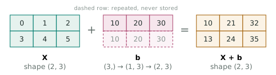
Broadcasting lets arrays of different shapes combine elementwise without copying. The rule fits in one sentence: line the shapes up from the right; along each axis the sizes must be equal, or one of them must be 1 (a missing leading axis counts as 1); the result takes the larger size. An axis of size 1 behaves as if it were repeated, but nothing is actually stored twice.

The most common case is adding a bias to every row of a batch. With $\mX \in \R^{N \times d}$ and $\vb \in \R^{d}$ , the sum $\mX + \vb$ adds $\vb$ to each row:

Figure B.1 Broadcasting treats a length-3 vector as shape (1, 3), then repeats that row to match (2, 3).

Listing B.3 Adding a bias is broadcasting

def add_bias(X, b):
    """X (N, d) + b (d,) -> (N, d): the same b is added to every row."""
    return X + b

Inserting axes of size 1 with None (an alias for np.newaxis) turns broadcasting into a tool for building all-pairs computations. To compare every row of $\mA \in \R^{N\times d}$ with every row of $\mB \in \R^{M\times d}$ , give them shapes (N, 1, d) and (1, M, d):

Listing B.4 All pairwise squared distances by broadcasting

def pairwise_squared_distances(A, B):
    """Rows A (N, d) and B (M, d) -> D (N, M) with D[i, j] = ||A[i] - B[j]||^2."""
    difference = A[:, None, :] - B[None, :, :]   # (N, 1, d) - (1, M, d) -> (N, M, d)
    return np.sum(difference ** 2, axis=-1)

The intermediate has shape (N, M, d), which is wasteful when d is large. Expanding the square avoids it:

\lVert \va_i - \vb_j \rVert^2 = \lVert \va_i \rVert^2 + \lVert \vb_j \rVert^2 - 2\, \va_i \cdot \vb_j\tag{B.1}

The last term for all pairs at once is a single matrix product, $\mA \mB^\T$ :

Listing B.5 The same distances with one matrix product

def pairwise_squared_distances_fast(A, B):
    """The same D without the (N, M, d) intermediate: ||a||^2 + ||b||^2 - 2 a.b."""
    squared_A = np.sum(A ** 2, axis=1)[:, None]      # (N, 1)
    squared_B = np.sum(B ** 2, axis=1)[None, :]      # (1, M)
    return squared_A + squared_B - 2 * A @ B.T       # (N, M)

Pitfall

A vector of shape (N,) is neither a row nor a column. Subtracting a column (N, 1) from it produces an (N, N) matrix, not an error. Assert shapes in your code; it costs nothing.

B.3 Reductions and `keepdims`

A reduction such as sum, mean, or max collapses one or more axes. Passing keepdims=True leaves each reduced axis in place with size 1, so the result broadcasts straight back against the input. Normalizing each row to sum to one is the canonical example:

Listing B.6 Reduce, keep the axis, broadcast back

def normalize_rows(X):
    """Scale each row of X (N, d) so that it sums to 1."""
    return X / np.sum(X, axis=1, keepdims=True)    # (N, d) / (N, 1)

Without keepdims, the row sums have shape (N,). They then align with the last axis of X, not the first: an error when N differs from d, and a silently wrong answer when N equals d (Exercise B.2).

Broadcasting and reduction are two faces of one idea, and backpropagation makes the link exact. If the forward pass copies a value to many places, the backward pass adds up the gradients arriving from those places. For $\mY = \mX + \vb$ with loss $L$ :

\frac{\partial L}{\partial b_j} = \sum_{i=1}^{N} \frac{\partial L}{\partial Y_{ij}} \qquad\text{so}\qquad \bar{\vb} = \sum_{i} \bar{\mY}_{i,:}\tag{B.2}

Here $\bar{\mY}$ denotes the gradient of $L$ with respect to $\mY$ . It has the same shape as $\mY$ (Section A.4). In general, the gradient of a broadcast input is the upstream gradient summed over every axis that broadcasting stretched:

Listing B.7 Summing a gradient back to the shape of a broadcast input

def unbroadcast(gradient, shape):
    """Sum a gradient over the axes that broadcasting stretched, returning `shape`."""
    extra = gradient.ndim - len(shape)
    gradient = gradient.sum(axis=tuple(range(extra))) if extra else gradient
    stretched = tuple(axis for axis, size in enumerate(shape)
                      if size == 1 and gradient.shape[axis] != 1)
    return gradient.sum(axis=stretched, keepdims=True) if stretched else gradient

unbroadcast lives in the book’s shared scratch package because the automatic differentiation chapter needs it for every elementwise operation.

B.4 Gather, scatter, and masks

Integer-array indexing gathers values. Two gathers appear in nearly every model. The first picks each example’s score for its true class, the heart of the cross-entropy loss:

Listing B.8 Gathering one entry per row

def true_class_scores(logits, labels):
    """logits (N, C), integer labels (N,) -> (N,) holding logits[i, labels[i]]."""
    return logits[np.arange(len(labels)), labels]

The second is an embedding lookup: a table of $V$ vectors, indexed by token IDs of any shape. Its gradient is the reverse operation, a scatter-add: each upstream gradient row is added into the table row of the token that produced it. When a token appears several times, its contributions must accumulate.

Listing B.9 An embedding lookup and its scatter-add gradient

def embedding_forward(table, ids):
    """table (V, d) and integer ids of any shape S -> vectors of shape S + (d,)."""
    return table[ids]


def embedding_backward(upstream, ids, vocabulary_size):
    """Gradient of the table: add each upstream vector into the row of its token."""
    gradient = np.zeros((vocabulary_size, upstream.shape[-1]), dtype=upstream.dtype)
    np.add.at(gradient, ids.reshape(-1), upstream.reshape(-1, upstream.shape[-1]))
    return gradient

Pitfall

gradient[ids] += upstream looks equivalent to np.add.at, but it is not. NumPy evaluates the right-hand side first, then assigns row by row, so a token that appears twice keeps only one contribution. Use np.add.at, or an equivalent matrix product (Exercise B.6).

Boolean arrays select and mask. The causal mask of a language model, which lets position $t$ look only at positions $s \le t$ , is a lower-triangular boolean matrix:

Listing B.10 A causal mask

def causal_mask(T):
    """mask[t, s] is True when position t may look at position s, i.e. s <= t."""
    return np.tril(np.ones((T, T), dtype=bool))

B.5 Batched products, heads, and `einsum`

The @ operator multiplies the last two axes and broadcasts over all the others. For stacks of matrices, shapes (…, n, k) @ (…, k, m) give (…, n, m).

Splitting a feature vector into heads is a reshape followed by a transpose. A reshape reinterprets the same memory with new axis sizes, taking entries in order. A transpose permutes axes by changing strides, without moving memory:

Listing B.11 Splitting a feature vector into heads, and merging them back

def split_heads(X, heads):
    """(B, T, H * d_h) -> (B, H, T, d_h): cut each feature vector into H chunks."""
    B, T, width = X.shape
    return X.reshape(B, T, heads, width // heads).transpose(0, 2, 1, 3)


def merge_heads(X):
    """(B, H, T, d_h) -> (B, T, H * d_h), the inverse of split_heads."""
    B, H, T, d_head = X.shape
    return X.transpose(0, 2, 1, 3).reshape(B, T, H * d_head)

The order matters. Reshaping (B, T, H·d_h) to (B, T, H, d_h) cuts each token’s vector into H consecutive chunks. Reshaping straight to (B, H, T, d_h) instead would deal the tokens' numbers out across heads like cards, mixing different tokens into one head (Exercise B.7).

np.einsum states a product by naming axes. An index that appears in the inputs but not in the output is summed over. Here it computes every query–key dot product, matching the matmul version:

Listing B.12 All-pairs dot products, two ways

def all_pair_dot_products(Q, K):
    """Q, K (B, H, T, d_h) -> S (B, H, T, T).

    S[b, h, t, s] is the dot product of query t with key s:
    Q[b, h, t] . K[b, h, s].
    """
    return np.einsum("bhtd,bhsd->bhts", Q, K)


def all_pair_dot_products_matmul(Q, K):
    return Q @ np.swapaxes(K, -1, -2)            # (..., T, d_h) @ (..., d_h, T)

B.6 Floating point

A binary floating-point number stores a sign, an exponent, and a fraction of $p$ bits. Numbers between two consecutive powers of two, $2^e \le |x| < 2^{e+1}$ , are spaced $2^{e-p}$ apart. The spacing is relative: the machine epsilon $\varepsilon = 2^{-p}$ is the gap just above 1. Rounding to the nearest representable number therefore makes a relative error of at most $\varepsilon / 2$ . The IEEE 754 standard [ieee754] fixes these formats; Goldberg [goldberg1991] remains the classic introduction.

Table B.1 Limits of the formats used in deep learning
Format	Exponent bits	Fraction bits	Machine epsilon	Largest value	Smallest normal
float64	11	52	$2^{-52} \approx 2.2 \times 10^{-16}$	$\approx 1.8 \times 10^{308}$	$\approx 2.2 \times 10^{-308}$
float32	8	23	$2^{-23} \approx 1.2 \times 10^{-7}$	$\approx 3.4 \times 10^{38}$	$\approx 1.2 \times 10^{-38}$
bfloat16	8	7	$2^{-7} \approx 7.8 \times 10^{-3}$	$\approx 3.4 \times 10^{38}$	$\approx 1.2 \times 10^{-38}$
float16	5	10	$2^{-10} \approx 9.8 \times 10^{-4}$	65504	$2^{-14} \approx 6.1 \times 10^{-5}$

Every format also has one sign bit. np.finfo reports these values for the formats NumPy supports:

Listing B.13 Reading the limits from NumPy

def float_limits():
    """Machine epsilon, largest value, and smallest normal value per dtype."""
    rows = []
    for dtype in (np.float16, np.float32, np.float64):
        info = np.finfo(dtype)
        rows.append((info.dtype.name, float(info.eps), float(info.max),
                     float(info.smallest_normal)))
    return rows

The two 16-bit formats trade differently. float16 spends bits on precision and runs out of range: $e^x$ overflows for $x > \ln 65504 \approx 11.09$ . bfloat16 keeps float32’s exponent, so it has the same range. The price is precision: only about three significant decimal digits [kalamkar2019]. NumPy has no bfloat16 type, so the book emulates it by rounding float32 values:

Listing B.14 Emulating bfloat16 rounding in float32

def round_to_bfloat16(x):
    """Round float32 values to the nearest bfloat16 (ties to even), returned as float32.

    bfloat16 keeps float32's sign bit and 8 exponent bits but only the top 7 of its
    23 fraction bits, so rounding happens on the low 16 bits of the float32 pattern.
    """
    bits = np.asarray(x, dtype=np.float32).view(np.uint32).astype(np.uint64)
    lsb = (bits >> 16) & 1  # the last kept bit decides ties
    rounded = ((bits + 0x7FFF + lsb) >> 16) << 16
    result = rounded.astype(np.uint32).view(np.float32)
    return np.where(np.isnan(x), np.float32(np.nan), result)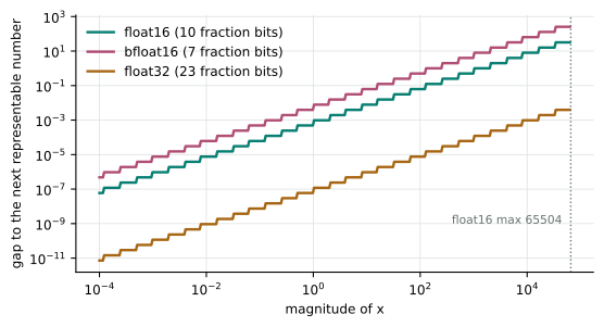

Spacing of representable numbers for float16

Figure B.2 The gap between neighbouring representable numbers grows in proportion to magnitude. Each format traces a staircase of slope one on log–log axes; fewer fraction bits shift it up.

Relative spacing explains the most important rule of mixed-precision training [micikevicius2017]: accumulate in float32. Adding a small number to a large running total loses it once the small number is under half the gap at the total’s magnitude. Adding 0.001 ten thousand times should give 10. A bfloat16 accumulator gets stuck at 0.5, where the gap is $2^{-8} \approx 0.0039$ . A float16 accumulator gets stuck at 4. A float32 accumulator reaches 10.0004 (Exercise B.8).

B.7 Numerical stability

Exponentials are the usual source of overflow. In float32, $e^{x}$ overflows for $x > 88.72$ . The fix is an exact identity (Higham [higham2002] treats such rearrangements systematically). For any constant $m$ ,

\logsumexp(\vz) = \log \sum_{i=1}^{n} e^{z_i} = m + \log \sum_{i=1}^{n} e^{z_i - m}.\tag{B.3}

Choosing $m = \max_i z_i$ makes every exponent non-positive, so nothing overflows. At least one term equals 1, so the sum inside the logarithm lies between 1 and $n$ . It also bounds the result:

\max_i z_i \;\le\; \logsumexp(\vz) \;\le\; \max_i z_i + \log n.\tag{B.4}

For $\vz = (1000, 1001, 1002)$ in float32, the naive formula returns inf; the shifted one returns 1002.4076. log_softmax follows by subtraction and is the numerically correct way to compute log-probabilities:

Listing B.15 A stable log-sum-exp and log-softmax

def logsumexp(z, axis=-1, keepdims=False):
    """log(sum(exp(z))) along `axis`, computed without overflow."""
    m = np.max(z, axis=axis, keepdims=True)
    m = np.where(np.isfinite(m), m, 0)        # all -inf rows: log(0) = -inf, not nan
    result = m + np.log(np.sum(np.exp(z - m), axis=axis, keepdims=True))
    return result if keepdims else np.squeeze(result, axis=axis)


def log_softmax(z, axis=-1):
    return z - logsumexp(z, axis=axis, keepdims=True)

The same idea protects the sigmoid and softplus. Evaluate them through $e^{-|x|}$ , which never exceeds 1:

\sigma(x) = \begin{cases} \dfrac{1}{1 + e^{-|x|}} & x \ge 0 \\[2ex] \dfrac{e^{-|x|}}{1 + e^{-|x|}} & x < 0 \end{cases} \qquad \log(1 + e^{x}) = \max(x, 0) + \log\!\left(1 + e^{-|x|}\right)\tag{B.5}

Listing B.16 Sigmoid and softplus without overflow

def sigmoid(x):
    """1 / (1 + exp(-x)) that never exponentiates a large positive number."""
    e = np.exp(-np.abs(x))                        # in (0, 1] for every x
    return np.where(x >= 0, 1 / (1 + e), e / (1 + e))


def softplus(x):
    """log(1 + exp(x)) = max(x, 0) + log(1 + exp(-|x|))."""
    return np.maximum(x, 0) + np.log1p(np.exp(-np.abs(x)))

np.log1p(u) and np.expm1(u) compute $\log(1+u)$ and $e^{u} - 1$ accurately for tiny $u$ , where the direct forms would round the small part away.

B.8 Checking gradients numerically

Every backward pass in this book is derived by hand, and every derivation is checked against a finite difference. For a scalar function, Taylor expansion on both sides of $x$ gives

\frac{f(x+h) - f(x-h)}{2h} = f'(x) + \frac{h^2}{6} f'''(\xi) \quad\text{for some } \xi \in (x - h,\, x + h).\tag{B.6}

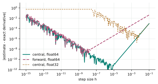
The even-order terms cancel, so the truncation error of this central difference shrinks like $h^2$ , against $h$ for the one-sided $(f(x+h) - f(x))/h$ . But each evaluation of $f$ is rounded by about $\varepsilon |f(x)|$ , and dividing by $2h$ amplifies that to $\varepsilon |f(x)| / h$ . The total error

E(h) \approx \frac{h^2}{6} |f'''(x)| + \frac{\varepsilon\, |f(x)|}{h}\tag{B.7}

is smallest near $h^\star = (3\varepsilon |f| / |f'''|)^{1/3}$ : about $10^{-5}$ in float64, with a best relative error near $10^{-11}$ . In float32 the best is only about $10^{-5}$ , too coarse to separate a correct gradient from a subtly wrong one, so gradient checks run in float64.

Finite-difference error against step size

Figure B.3 Error of finite-difference estimates of the derivative of sin at 1. Moving left, truncation error falls until round-off takes over. Central differences reach a far lower floor, and float32 bottoms out about six orders of magnitude above float64.

For an array input, perturb one entry at a time, on a float64 copy so the check never disturbs its input:

Listing B.17 Central-difference gradients, from the shared scratch package

def numerical_gradient(f, x, h=1e-5):
    """Central-difference estimate of the gradient of a scalar function f at x."""
    x = np.array(x, dtype=np.float64)  # a float64 copy: never perturb the caller's x
    gradient = np.zeros_like(x)
    for index in np.ndindex(x.shape):
        original = x[index]
        x[index] = original + h
        plus = f(x)
        x[index] = original - h
        minus = f(x)
        x[index] = original
        gradient[index] = (plus - minus) / (2 * h)
    return gradient

Compare with a relative error, because gradients range over many orders of magnitude:

\operatorname{err}(\va, \vn) = \max_i \frac{|a_i - n_i|}{|a_i| + |n_i|}\tag{B.8}

Listing B.18 Relative error, guarded against division by zero

def relative_error(a, b, floor=1e-12):
    """Largest elementwise |a - b| / (|a| + |b|), guarded against 0 / 0."""
    a = np.asarray(a, dtype=np.float64)
    b = np.asarray(b, dtype=np.float64)
    return float(np.max(np.abs(a - b) / np.maximum(np.abs(a) + np.abs(b), floor)))

A correct float64 gradient typically scores below $10^{-7}$ and a wrong one above $10^{-3}$ . For a function returning an array $\mY$ , check the scalar $L = \sum_{ij} G_{ij} Y_{ij}$ for a fixed random $\mG$ : its gradient is the backward pass with upstream gradient $\mG$ .

Listing B.19 The check used throughout the book

def check_gradient(f, x, analytic, h=1e-5, tolerance=1e-7):
    """Raise if an analytic gradient disagrees with central differences."""
    error = relative_error(analytic, numerical_gradient(f, x, h))
    if error > tolerance:
        raise AssertionError(f"gradient check failed: relative error {error:.2e}"
                             f" > {tolerance:.0e}")
    return error

In practice

Kinks break finite differences. If a ReLU input lies within $h$ of zero, the two sides of the difference straddle the kink and the estimate is meaningless. Draw test inputs away from kinks, or check at a few random points. Keep the arrays tiny: the check costs two function evaluations per entry.

Key equations

Broadcasting: align shapes from the right; sizes must match or be 1. The gradient of a broadcast input is the upstream gradient summed over the stretched axes.

\logsumexp(\vz) = m + \log \sum_i e^{z_i - m}, \quad m = \max_i z_i

\max_i z_i \le \logsumexp(\vz) \le \max_i z_i + \log n

\log(1 + e^{x}) = \max(x, 0) + \log(1 + e^{-|x|})

f'(x) \approx \frac{f(x+h) - f(x-h)}{2h}, \qquad \text{error} = O(h^2) + O(\varepsilon / h)

Machine epsilon: float32 $2^{-23}$ , bfloat16 $2^{-7}$ , float16 $2^{-10}$ , float64 $2^{-52}$ .

B.9 Teach it

The one-sentence version. NumPy code for deep learning is shape bookkeeping. Get the shapes right, respect the finite precision of floats, and check every gradient against a finite difference.

An analogy for broadcasting. Think of a rubber stamp. The bias vector is a stamp one row tall. Broadcasting presses it onto every row of the batch. The backward pass asks how much each part of the stamp contributed, and the answer is the total of the ink it left on every row.

At the board.

Write two shapes right-aligned, (4, 1, 3) over (5, 1), and fill the missing axis with a 1.
Compare column by column: 3 with 1, 1 with 5, 4 with 1. Circle every 1 that stretches, and read off the result (4, 5, 3).
Write $Y_{ij} = X_{ij} + b_j$ and ask which entries of $\mY$ depend on $b_2$ . The answer, a whole column, turns the chain rule into a column sum.
Show $e^{1000}$ overflowing. Then factor out $e^{1000}$ and write the log-sum-exp identity.
Sketch the U-shaped error curve of the finite difference, labelling the truncation and round-off sides.

Misconceptions to address.

"A (N,) array is a row vector." It has one axis. It broadcasts as a row, (1, N), which is exactly how it combines with a column into an (N, N) matrix.
"`x[idx] += y` accumulates duplicates." It does not; use np.add.at.
"Smaller $h$ is always better." Below the optimum, round-off error grows as $1/h$ .
"float16 and bfloat16 are interchangeable." One runs out of range and the other runs out of precision.

Check for understanding. Why does reshape(B, H, T, d_h) on a (B, T, H·d_h) array produce garbage, while reshape(B, T, H, d_h) followed by a transpose does not?

B.10 Exercises

Exercise B.1 ★ Predict the shape

Let A, B, C, and D have shapes (4, 1, 3), (5, 1), (3,), and (4, 3). Give the shape of A + B, A + C, B + C, and A * D, and explain why D + B fails.

Solution in Appendix D

Exercise B.2 ★ The missing keepdims

A colleague normalizes rows with X / X.sum(axis=1) where X has shape (N, d). When does this raise an error? When does it run but return the wrong answer, and what does it compute instead?

Solution in Appendix D

Exercise B.3 ★★ Why summing is right

For $\mY = \mX + \vb$ with $\mX \in \R^{N \times d}$ and $\vb \in \R^{d}$ , derive (B.2) from the chain rule. Then argue that unbroadcast is correct for any broadcast. Hint: show that $\langle \operatorname{broadcast}(\vv), \mG \rangle = \langle \vv, \operatorname{unbroadcast}(\mG) \rangle$ for every $\vv$ and $\mG$ .

Solution in Appendix D

Exercise B.4 ★★ Log-sum-exp

Prove the shift identity (B.3) and the bounds (B.4). Then show that the gradient of $\logsumexp(\vz)$ with respect to $\vz$ is $\softmax(\vz)$ .

Solution in Appendix D

Exercise B.5 ★★ Choosing the step

Starting from Taylor expansions of $f(x+h)$ and $f(x-h)$ , derive (B.6). Minimize (B.7) over $h$ , and estimate the best achievable error in float32 and in float64.

Solution in Appendix D

Exercise B.6 ★★★ Three embedding gradients

Implement the embedding-table gradient three ways: with a Python loop, with np.add.at, and as a matrix product with a one-hot matrix. Show that all three agree, and that gradient[ids] += upstream does not when an ID repeats. Which rows does the buggy version get right?

Solution in Appendix D

Exercise B.7 ★★★ The wrong reshape

Write split_heads_wrong(X, heads), which reshapes (B, T, H·d_h) directly to (B, H, T, d_h). Find a small input where it disagrees with split_heads, and explain the difference in terms of memory order.

Solution in Appendix D

Exercise B.8 ★★★ Where a sum stalls

Use round_to_bfloat16 to add 0.001 to a running total 10,000 times, rounding after every step. Repeat with float16 and float32 accumulators. Explain the value at which each low-precision sum stops growing.

Solution in Appendix D

References

[harris2020] C. R. Harris et al. Array programming with NumPy. Nature 585, 357–362, 2020. arXiv:2006.10256
[goldberg1991] D. Goldberg. What every computer scientist should know about floating-point arithmetic. ACM Computing Surveys 23(1), 5–48, 1991.
[higham2002] N. J. Higham. Accuracy and Stability of Numerical Algorithms, 2nd edition. SIAM, 2002.
[ieee754] IEEE Standard for Floating-Point Arithmetic, IEEE 754-2019.
[kalamkar2019] D. Kalamkar et al. A study of BFLOAT16 for deep learning training. 2019. arXiv:1905.12322
[micikevicius2017] P. Micikevicius et al. Mixed precision training. ICLR 2018. arXiv:1710.03740

B.1 Arrays, dtypes, and views

B.2 Broadcasting

B.3 Reductions and keepdims

B.4 Gather, scatter, and masks

B.5 Batched products, heads, and einsum

B.6 Floating point

B.7 Numerical stability

B.8 Checking gradients numerically

B.9 Teach it

B.10 Exercises

References

B.3 Reductions and `keepdims`

B.5 Batched products, heads, and `einsum`