Probability Theory | ML Refresher

6.1 Random variables and distributions

A random variable is a quantity whose value is uncertain: the label of the next training example, the next token of a sentence, a weight at initialization. Its distribution says how likely each value is. Probabilities obey three rules, the Kolmogorov axioms: every event has probability at least 0; the event "something happens" has probability 1; and the probabilities of mutually exclusive events add.

A discrete random variable takes countably many values, and its probability mass function $p(x) = P(X = x)$ sums to 1. A continuous random variable, such as a real weight, has a probability density function $p(x)$ that integrates to 1. The two look alike on paper, but they mean different things:

P(a < X < b) = \int_a^b p(x)\, \dd x .\tag{6.1}

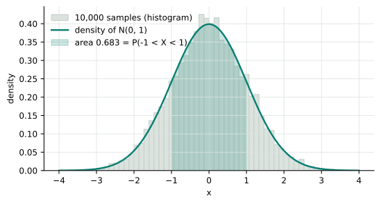
A density is a height, not a probability. Probability is area under the density, and the probability of any single exact value is zero. A density can therefore exceed 1: a Gaussian with standard deviation 0.1 has density 3.99 at its mean, while the probability of landing within 0.05 of the mean is only 0.383 (Exercise 6.1). The cumulative distribution function $F(x) = P(X \le x)$ turns areas into differences: $P(a < X < b) = F(b) - F(a)$ .

Five distributions cover almost everything in this book:

Table 6.1 Distributions used throughout the book
Distribution	Values	Probability or density	Mean, variance
Bernoulli( $p$ )	$x \in \{0, 1\}$	$p^{x}(1-p)^{1-x}$	$p, \; p(1-p)$
Categorical( $\vpi$ )	$x \in \{1, \dots, K\}$	$\pi_x$ , with $\sum_k \pi_k = 1$	(a label, not a number)
Uniform( $a, b$ )	$a \le x \le b$	$1/(b - a)$	$\tfrac{a+b}{2}, \; \tfrac{(b-a)^2}{12}$
Gaussian $\mathcal{N}(\mu, \sigma^2)$	$x \in \R$	$\tfrac{1}{\sigma\sqrt{2\pi}} e^{-(x-\mu)^2 / (2\sigma^2)}$	$\mu, \; \sigma^2$
Gaussian $\mathcal{N}(\vmu, \mSigma)$	$\vx \in \R^d$	$\tfrac{e^{-\frac12 (\vx-\vmu)^\T \mSigma^{-1} (\vx-\vmu)}}{\sqrt{(2\pi)^d \det \mSigma}}$	$\vmu, \; \mSigma$

The categorical distribution is the one to know best. A classifier’s softmax output is a categorical distribution over classes, and a language model’s output is a categorical distribution over tokens.

Listing 6.1 Probability mass and density functions

def bernoulli_pmf(x, p):
    """P(X = x) for x in {0, 1} when X ~ Bernoulli(p)."""
    return np.where(x == 1, p, 1 - p)


def gaussian_pdf(x, mean, std):
    """Density of N(mean, std^2) at x: a height, not a probability."""
    z = (x - mean) / std
    return np.exp(-0.5 * z ** 2) / (std * np.sqrt(2 * np.pi))


def gaussian_log_pdf(x, mean, std):
    """log of gaussian_pdf, computed without exponentiating."""
    z = (x - mean) / std
    return -0.5 * z ** 2 - np.log(std) - 0.5 * np.log(2 * np.pi)

The log density avoids computing an exponential only to take its logarithm again. Working with log-probabilities is the norm in deep learning: probabilities of long sequences underflow float32 quickly, while their logarithms simply add.

Histogram of Gaussian samples against the Gaussian density

Figure 6.1 A histogram of samples approaches the density. The shaded area is a probability; the height of the curve is not.

6.2 Joint, marginal, and conditional distributions

Two random variables $X$ and $Y$ have a joint distribution $p(x, y)$ . For discrete variables it is a table. Summing out one variable gives the other’s marginal distribution, and dividing the joint by a marginal gives a conditional distribution:

p(x) = \sum_y p(x, y), \qquad p(y \mid x) = \frac{p(x, y)}{p(x)} .\tag{6.2}

In array terms, a marginal is a sum over an axis and a conditional is a row normalized to sum to one, the same keepdims pattern as in Section B.3:

Listing 6.2 Marginals and conditionals of a joint table

def marginals(joint):
    """joint[i, j] = P(X = i, Y = j) -> (P(X = i) for each i, P(Y = j) for each j)."""
    return joint.sum(axis=1), joint.sum(axis=0)


def conditional_y_given_x(joint):
    """Row i holds P(Y = j | X = i): each row of the joint, renormalized."""
    return joint / joint.sum(axis=1, keepdims=True)

Rearranging the definition gives the product rule, $p(x, y) = p(x)\, p(y \mid x)$ . Applied repeatedly, it factorizes any joint distribution over a sequence:

p(x_1, x_2, \dots, x_T) = \prod_{t=1}^{T} p(x_t \mid x_1, \dots, x_{t-1}) .\tag{6.3}

This chain rule of probability is exact and involves no assumptions. It is also the blueprint of every autoregressive language model: learn $p(x_t \mid x_{<t})$ , the distribution of the next token given all previous ones, and the probability of an entire text is the product.

$X$ and $Y$ are independent when $p(x, y) = p(x)\, p(y)$ for all $x, y$ : knowing one tells you nothing about the other. Training examples are usually modelled as independent and identically distributed (i.i.d.) draws from one unknown distribution.

6.2.1 Bayes' rule

Writing the product rule both ways, $p(h)\, p(e \mid h) = p(e)\, p(h \mid e)$ , and dividing gives Bayes' rule. It turns the probability of evidence $e$ given a hypothesis $h$ into the probability of the hypothesis given the evidence:

p(h \mid e) = \frac{p(e \mid h)\, p(h)}{\sum_{h'} p(e \mid h')\, p(h')} .\tag{6.4}

The denominator is just the sum of the numerator over all hypotheses, so in code Bayes' rule is "multiply, then normalize":

Listing 6.3 Bayes' rule over a list of hypotheses

def posterior(prior, likelihood):
    """P(H = h | evidence) from priors P(H = h) and likelihoods P(evidence | H = h)."""
    unnormalized = prior * likelihood       # P(H = h, evidence)
    return unnormalized / unnormalized.sum()  # divide by P(evidence)

A detector for machine-generated essays catches 95% of generated essays and wrongly flags 5% of human-written ones. If 1% of submitted essays are generated, what is the probability that a flagged essay is generated? The flagged essays are 0.0095 generated and 0.0495 human, so the answer is $0.0095 / 0.059 \approx 0.16$ . A flag is mostly wrong, because the rare class is rare. Getting this base-rate effect wrong is the most common mistake in reasoning about classifiers (Exercise 6.2).

6.3 Expectation and variance

The expectation of a function of a random variable is its probability-weighted average:

\E[f(X)] = \sum_x f(x)\, p(x) \quad\text{or}\quad \E[f(X)] = \int f(x)\, p(x)\, \dd x .\tag{6.5}

Training objectives are expectations: the expected loss over the data distribution, or the expected reward of a policy. Expectation is linear, $\E[aX + bY] = a\E[X] + b\E[Y]$ , whether or not $X$ and $Y$ are independent. That makes it the most useful identity in this chapter.

Variance measures spread around the mean, and covariance measures how two variables move together:

\begin{aligned} \Var[X] &= \E\big[(X - \E[X])^2\big] = \E[X^2] - \E[X]^2, \\ \Cov[X, Y] &= \E\big[(X - \E[X])(Y - \E[Y])\big] . \end{aligned}\tag{6.6}

Unlike expectation, variance is not linear. $\Var[aX + b] = a^2 \Var[X]$ , and $\Var[X + Y] = \Var[X] + \Var[Y] + 2\Cov[X, Y]$ . For i.i.d. variables with variance $\sigma^2$ , the covariances vanish and the mean of $n$ of them has

\Var\Big[\frac{1}{n} \sum_{i=1}^{n} X_i\Big] = \frac{\sigma^2}{n} .\tag{6.7}

This one line explains two facts about training. First, a minibatch gradient is an average over examples, so its noise shrinks like $1/\sqrt{B}$ in the batch size $B$ : four times the batch halves the noise. Second, the variance of a sum of $n$ independent terms grows like $n$ . That is why weights are initialized with variance proportional to $1/n$ : then a sum of $n$ weighted inputs keeps a stable scale from layer to layer.

For a random vector $\vx \in \R^d$ , the covariance matrix $\mSigma$ collects all pairwise covariances, $\Sigma_{ij} = \Cov[x_i, x_j]$ .

6.4 Monte Carlo estimation

Most expectations in deep learning cannot be computed exactly: the sum runs over every possible image or sentence. Instead, draw $n$ samples and average:

\E[f(X)] \approx \frac{1}{n} \sum_{i=1}^{n} f(x_i), \qquad x_i \sim p .\tag{6.8}

The estimate is unbiased: its expectation is exactly $\E[f(X)]$ . By (6.7), its standard deviation, the standard error, is $\sigma_f / \sqrt{n}$ . The law of large numbers guarantees that the average converges to the expectation. The central limit theorem adds that, for large $n$ , the error is approximately Gaussian, so the estimate lies within two standard errors about 95% of the time.

Listing 6.4 A Monte Carlo estimate with its standard error

def monte_carlo(f, sample, n, rng):
    """Estimate E[f(X)] from n draws, and the standard error of that estimate."""
    values = f(sample(n, rng))
    return values.mean(), values.std(ddof=1) / np.sqrt(n)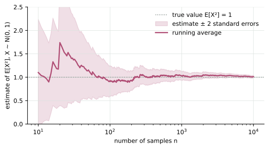

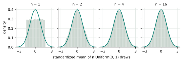
A running Monte Carlo average converging to 1 inside a narrowing band

Figure 6.2 The running Monte Carlo estimate of

\E[X^2]

for standard Gaussian

X

. The band narrows like

1/\sqrt{n}

: a hundred times more samples buy one more correct digit.

Histograms of means of uniform draws becoming Gaussian

Figure 6.3 Means of

n

uniform draws, standardized. Even a flat distribution produces Gaussian-looking averages by

n = 16

.

Stochastic gradient descent is Monte Carlo estimation. The gradient of the average loss over the training set is an expectation over examples, and a minibatch gradient is its unbiased estimate from a random sample.

6.4.1 Gradients of expectations

Reinforcement learning, and much of generative modelling, needs the gradient of an expectation with respect to the parameters of the distribution itself: $\nabla_\theta \E_{x \sim p_\theta}[f(x)]$ . The samples depend on $\theta$ , so we cannot simply differentiate inside the average. For a discrete distribution, move the gradient inside the sum and use $\nabla p = p \nabla \log p$ :

\nabla_\theta \E_{x \sim p_\theta}[f(x)] = \sum_x f(x) \nabla_\theta p_\theta(x) = \E_{x \sim p_\theta}\big[f(x)\, \nabla_\theta \log p_\theta(x)\big] .\tag{6.9}

This is the score-function or log-derivative estimator, and REINFORCE is its name in reinforcement learning [williams1992]. It needs only samples and the gradient of $\log p_\theta$ , not the gradient of $f$ . That matters when $f$ is a reward computed by a program, a test suite, or a human. The same identity holds for densities.

When the sample can instead be written as a differentiable function of the parameters and parameter-free noise, $x = \mu + \sigma\varepsilon$ with $\varepsilon \sim \mathcal{N}(0, 1)$ , the gradient passes through the sample. This reparameterization estimator is $\E_\varepsilon[f'(\mu + \sigma\varepsilon)]$ [kingma2013]:

Listing 6.5 Two unbiased estimators of the same gradient

def score_function_gradient(f, mean, std, n, rng):
    """d/d(mean) of E[f(X)], X ~ N(mean, std^2), as the average of f(x) * score(x)."""
    x = mean + std * rng.standard_normal(n)
    score = (x - mean) / std ** 2              # d log p(x) / d mean
    return np.mean(f(x) * score)


def reparameterized_gradient(df, mean, std, n, rng):
    """The same derivative through x = mean + std * eps: the average of f'(x)."""
    x = mean + std * rng.standard_normal(n)
    return np.mean(df(x))

Both are unbiased, but their variances differ. For $f(x) = x^2$ at $\mu = \sigma = 1$ , the true derivative is 2. The per-sample variance is 30 for the score-function estimator and 4 for the reparameterized one. Subtracting a constant baseline from $f$ keeps the score function unbiased, because $\E[\nabla_\theta \log p_\theta(x)] = 0$ . With the baseline $\E[f(X)] = 2$ , the variance falls from 30 to 18 (Exercise 6.6). Every policy-gradient method in the reinforcement-learning chapters is this estimator plus a cleverer baseline.

6.5 Maximum likelihood

A model is a family of distributions $p_\vtheta$ indexed by parameters. Given i.i.d. data $x_1, \dots, x_N$ , the likelihood of $\vtheta$ is the probability the model assigns to that data. Maximum likelihood estimation (MLE) picks the parameters that make the data most probable. Products of many probabilities underflow and are awkward to differentiate, so we minimize the average negative log-likelihood instead:

\hat{\vtheta} = \argmin_{\vtheta} \; -\frac{1}{N} \sum_{i=1}^{N} \log p_\vtheta(x_i) .\tag{6.10}

For a coin with $k$ heads in $N$ flips, setting the derivative of $-k \log p - (N - k)\log(1-p)$ to zero gives $\hat{p} = k / N$ . For a Gaussian, the maximum-likelihood mean is the sample mean and the variance is the mean squared deviation (Exercise 6.4):

Listing 6.6 Maximum likelihood for a Gaussian

def gaussian_mle(x):
    """Maximum-likelihood mean and standard deviation of 1-D samples."""
    mean = x.mean()
    return mean, np.sqrt(np.mean((x - mean) ** 2))    # divides by n, not n - 1


def gaussian_nll(x, mean, std):
    """Average negative log-likelihood of samples x under N(mean, std^2)."""
    return -np.mean(gaussian_log_pdf(x, mean, std))

The most important use of MLE is conditional: the model predicts a distribution over targets $y$ given inputs $x$ , and training minimizes $-\frac{1}{N}\sum_i \log p_\vtheta(y_i \mid x_i)$ . Choosing that distribution is choosing the loss:

\begin{aligned} y \sim \mathcal{N}(\hat{y}, \sigma^2) &\;\Longrightarrow\; -\log p = \tfrac{1}{2\sigma^2}(y - \hat{y})^2 + \log \sigma + \tfrac12 \log 2\pi \\ y \sim \text{Bernoulli}(\hat{p}) &\;\Longrightarrow\; -\log p = -y \log \hat{p} - (1 - y)\log(1 - \hat{p}) \\ y \sim \text{Categorical}(\hat{\vpi}) &\;\Longrightarrow\; -\log p = -\log \hat{\pi}_y \end{aligned}\tag{6.11}

Mean squared error is Gaussian maximum likelihood with a fixed variance. Binary cross-entropy is Bernoulli maximum likelihood. Cross-entropy for classification, and the pretraining loss of every language model, is categorical maximum likelihood.

Listing 6.7 Three familiar losses, written as negative log-likelihoods

def gaussian_regression_nll(y, prediction, std=1.0):
    """Targets y ~ N(prediction, std^2): mean squared error / (2 std^2) + constant."""
    return -np.mean(gaussian_log_pdf(y, prediction, std))


def bernoulli_nll(y, p):
    """Binary labels y ~ Bernoulli(p): the binary cross-entropy."""
    return -np.mean(y * np.log(p) + (1 - y) * np.log(1 - p))


def categorical_nll(labels, probabilities):
    """Class labels ~ Categorical(probabilities[i]): the cross-entropy."""
    return -np.mean(np.log(probabilities[np.arange(len(labels)), labels]))

6.6 Sampling

Every sampler starts from uniform random numbers in $[0, 1)$ and transforms them. The inverse-CDF method is the most direct transformation. If $U$ is uniform and $F$ is a continuous CDF, then $F^{-1}(U)$ has CDF $F$ , because $P(F^{-1}(U) \le x) = P(U \le F(x)) = F(x)$ . For the exponential distribution, $F(x) = 1 - e^{-\lambda x}$ inverts in closed form:

Listing 6.8 Inverse-CDF sampling

def sample_exponential(rate, n, rng):
    """Invert F(x) = 1 - exp(-rate * x): x = -log(1 - u) / rate for uniform u."""
    return -np.log1p(-rng.random(n)) / rate

For a categorical distribution, the CDF is a cumulative sum, and inverting it means finding the first cumulative total that exceeds a uniform draw. This is how a language model picks its next token once it has computed the probabilities. The book’s shared scratch package provides a batched version, one draw per row:

Listing 6.9 Sampling from a categorical distribution

def sample_categorical(probabilities, rng):
    """One draw per row: probabilities (..., K) -> indices (...,).

    Inverts the cumulative distribution: index i is chosen when
    cumulative[i - 1] <= u < cumulative[i] for a uniform u.
    """
    cumulative = np.cumsum(probabilities, axis=-1)
    total = cumulative[..., -1:]                      # 1 up to rounding
    u = rng.random(cumulative.shape[:-1] + (1,)) * total
    return np.sum(cumulative <= u, axis=-1)

The Gumbel-max trick samples a categorical distribution from its logits, the unnormalized log-probabilities $z_k$ with $\pi_k \propto e^{z_k}$ . Add independent Gumbel noise $g_k = -\log(-\log u_k)$ to each logit and take the argmax:

\argmax_k \big(z_k + g_k\big) \sim \text{Categorical}\big(\softmax(\vz)\big) .\tag{6.12}

Listing 6.10 The Gumbel-max trick

def sample_gumbel_max(logits, rng):
    """argmax(logits + Gumbel noise) is one draw from softmax(logits), per row."""
    u = rng.uniform(np.finfo(np.float64).tiny, 1.0, size=np.shape(logits))
    gumbel = -np.log(-np.log(u))
    return np.argmax(logits + gumbel, axis=-1)

It never normalizes, which makes it convenient for sampling in parallel and for search. Its continuous relaxation, the Gumbel-softmax, lets gradients flow through discrete choices [maddison2014] [jang2016]. Dividing the logits by a temperature $T$ before adding noise samples $\softmax(\vz / T)$ : sharper for $T < 1$ , flatter for $T > 1$ (Exercise 6.7).

In practice

A language model’s output layer produces one logit per vocabulary entry. Llama 3’s vocabulary, for example, has 128K tokens [grattafiori2024]. Pretraining minimizes the categorical negative log-likelihood of each next token, (6.3) turned into a loss. Generation samples from the resulting distribution, usually after reshaping it with a temperature or truncation. Dropout draws Bernoulli masks, minibatches are Monte Carlo samples of the data, and reinforcement-learning fine-tuning methods such as PPO and GRPO are score-function estimators with learned or group-average baselines [shao2024].

Key equations

P(a < X < b) = \int_a^b p(x)\,\dd x, \qquad p(y \mid x) = \frac{p(x, y)}{p(x)}, \qquad p(h \mid e) \propto p(e \mid h)\, p(h)

p(x_1, \dots, x_T) = \prod_t p(x_t \mid x_{<t})

\E[aX + bY] = a\E[X] + b\E[Y], \qquad \Var[X] = \E[X^2] - \E[X]^2, \qquad \Var[\bar{X}_n] = \sigma^2 / n

\nabla_\theta \E_{p_\theta}[f(x)] = \E_{p_\theta}[f(x)\, \nabla_\theta \log p_\theta(x)]

\hat{\vtheta} = \argmin_\vtheta -\tfrac1N \textstyle\sum_i \log p_\vtheta(y_i \mid x_i); \quad \text{Gaussian} \to \text{MSE}, \; \text{Categorical} \to \text{cross-entropy}

\argmax_k (z_k + g_k) \sim \softmax(\vz), \qquad g_k = -\log(-\log u_k)

6.7 Teach it

The one-sentence version. A model outputs a probability distribution, training makes the observed data likely under it, and generation draws samples from it.

An analogy for densities. Population density is people per square kilometre. A tiny town can have a density far higher than a country’s, yet contain fewer people. You count people by multiplying density by area. A probability density works the same way: probability is density times width, or area under the curve.

At the board.

Draw a 2×2 joint table (the one in the tests: 0.30, 0.10, 0.15, 0.45). Sum the rows and columns to get the marginals in the margins, which is where the name comes from.
Divide a row by its total to get a conditional. Then run the machine-generated essay example through a tree of 10,000 essays, and let the audience find the 16%.
Write $p(x_1, x_2, x_3) = p(x_1)\, p(x_2 \mid x_1)\, p(x_3 \mid x_1, x_2)$ and say: this is a language model.
Take ten coin flips with seven heads. Plot the log-likelihood against $p$ and show the peak at 0.7. Then write the Gaussian log-likelihood and let squared error fall out of it.

Misconceptions to address.

"A probability density can’t exceed 1." Only its integral is bounded.
" $P(A \mid B) = P(B \mid A)$ ." Confusing these is the base-rate fallacy.
"Uncorrelated means independent." Zero covariance rules out only linear dependence: $X$ and $X^2$ are uncorrelated for symmetric $X$ , yet completely dependent.
"Sampling a model means taking its most likely output." That is decoding by argmax, and it produces repetitive text. Sampling draws in proportion to probability.

Check for understanding. Why does doubling the batch size not halve the noise in a minibatch gradient?

6.8 Exercises

Exercise 6.1 ★ A density above one

Compute the density of $\mathcal{N}(0, 0.1^2)$ at 0, and the probability that a draw lands within 0.05 of 0. Explain why the first number can exceed 1 while the second cannot.

Solution in Appendix D

Exercise 6.2 ★ Base rates

Repeat the machine-generated essay calculation from Section 6.2 for a course in which 20% of essays are generated, with the same detector. Why does the answer change so much, although the detector is unchanged?

Solution in Appendix D

Exercise 6.3 ★★ When averaging stops helping

Prove (6.7) for i.i.d. draws. Then suppose each pair of draws has correlation $\rho$ . Show that the variance of the mean is $\sigma^2(\rho + (1 - \rho)/n)$ , and explain what this means for a minibatch built from near-duplicate examples.

Solution in Appendix D

Exercise 6.4 ★★ Gaussian maximum likelihood

Derive the maximum-likelihood estimates $\hat\mu$ and $\hat\sigma^2$ for i.i.d. Gaussian data by setting the gradient of the negative log-likelihood to zero. Then show that $\E[\hat\sigma^2] = \frac{n-1}{n}\sigma^2$ .

Solution in Appendix D

Exercise 6.5 ★★ Losses from noise models

Show that minimizing the Gaussian negative log-likelihood with a fixed $\sigma$ is equivalent to minimizing mean squared error. Which loss results if the noise is Laplace, $p(y \mid \hat{y}) = \frac{1}{2b} e^{-|y - \hat{y}|/b}$ ? What does each loss predict for a target distribution with outliers?

Solution in Appendix D

Exercise 6.6 ★★ The score function and its baseline

Derive (6.9) for a discrete distribution. Show that $\E_{p_\theta}[\nabla_\theta \log p_\theta(x)] = 0$ , and conclude that subtracting any constant baseline from $f$ leaves the estimator unbiased. For $x \sim \mathcal{N}(1, 1)$ and $f(x) = x^2$ , verify the per-sample variances 30, 18, and 4 quoted in Section 6.4.1.

Solution in Appendix D

Exercise 6.7 ★★★ Why Gumbel-max works

Prove (6.12). Hint: the CDF of a standard Gumbel variable is $e^{-e^{-g}}$ ; compute the probability that $z_k + g_k$ exceeds every other $z_j + g_j$ by conditioning on $g_k$ . Then check it empirically, and show that dividing the logits by $T$ before adding the noise samples $\softmax(\vz / T)$ .

Solution in Appendix D

Exercise 6.8 ★★★ Designing a sampler

Use the inverse-CDF method to sample from the density $p(x) = 2x$ on $[0, 1]$ . Check that the sample mean approaches 2/3 and that a quarter of the samples fall below 1/2.

Solution in Appendix D

References

[blitzstein2019] J. K. Blitzstein and J. Hwang. Introduction to Probability, 2nd edition. CRC Press, 2019. https://projects.iq.harvard.edu/stat110
[bishop2006] C. M. Bishop. Pattern Recognition and Machine Learning. Springer, 2006.
[grattafiori2024] A. Grattafiori et al. The Llama 3 herd of models. 2024. arXiv:2407.21783
[jang2016] E. Jang, S. Gu, and B. Poole. Categorical reparameterization with Gumbel-softmax. ICLR 2017. arXiv:1611.01144
[kingma2013] D. P. Kingma and M. Welling. Auto-encoding variational Bayes. ICLR 2014. arXiv:1312.6114
[maddison2014] C. J. Maddison, D. Tarlow, and T. Minka. A* sampling. NeurIPS 2014. arXiv:1411.0030
[shao2024] Z. Shao et al. DeepSeekMath: Pushing the limits of mathematical reasoning in open language models. 2024. arXiv:2402.03300
[williams1992] R. J. Williams. Simple statistical gradient-following algorithms for connectionist reinforcement learning. Machine Learning 8, 229–256, 1992.